Window Functions in SQL
- Ekta Aggarwal

- Jul 24, 2022
- 7 min read
In this tutorial we will learn about window functions in SQL
To understand window functions, you can imagine that you do a calculation on a subset (or maybe full dataset) dataset, i.e., you are creating a window and then you map that calculation (window) to the original or grouped dataset. The best way to learn about window functions are with help of several tasks.
Following window functions would be covered in this tutorial:
Dataset:
For this tutorial we shall make use of the data: sales_table
CREATE TABLE sales_table(
Date date,
SKU_ID int,
SKU_Name varchar(100),
Category varchar(20),
Sales float,
Quantity int)
INSERT INTO
sales_table(Date,SKU_ID,Category,SKU_Name,Sales, Quantity)
VALUES
('1Jan2022',1001,'Cosmetics','Maybelline Hyper gloss Eyeliner',15,1),
('1Jan2022',1002,'Groceries','Bread',1.89,2),
('1Jan2022',1004,'Biscuits','McVities Digestive',17.9,10),
('1Jan2022',1005,'Chocolate','Malteasers',19.99,20),
('1Jan2022',1001,'Cosmetics','Maybelline Hyper gloss Eyeliner',9.99,1),
('1Jan2022',1002,'Groceries','Bread',1.05,1),
('1Jan2022',1002,'Groceries','Bread',7.12,5),
('2Jan2022',1004,'Biscuits','McVities Digestive',0.88,1),
('2Jan2022',1005,'Chocolate','Malteasers',9.99,10),
('2Jan2022',1004,'Biscuits','McVities Digestive',0.88,1),
('2Jan2022',1005,'Chocolate','Malteasers',6.99,5);Our data looks as follows:
In our data we have got sales information of different products on different dates.
SELECT * FROM sales_table;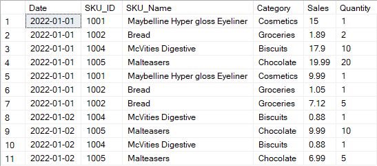
OVER:
Task: To get the total sales for entire data along with existing data as new column:
If I had to use subqueries then I would use the following code, where firstly I am selecting all the columns and creating a subquery to create our new column total_sales
SELECT * , (select sum(sales) from sales_table) as total_sales from sales_table;But since subqueries can be complex, thus as an alternative, we can use OVER( ) clause.
OVER( ) statement can be understood by 2 steps:
Step 1: OVER( ) clause goes through all the rows in the dataset (unless something is specified in inside OVER( ) statement) and does some calculation for that set of the data - which forms a temporary window. .
Step 2: Then the new window is joined to the original or some grouped dataset.
Step 1: In the code below, we are calculating sum(sales) for all the rows using OVER( ) statement.
Step 2: Then it joins the new column of total_sales to the original sales_table.
SELECT * , sum(sales) over() as total_sales
FROM sales_table;
In the output below you can see that the last column of total_sales for entire dataset has been added.

WHERE statement in a query with OVER( ) clause:
If we use a WHERE statement in a SQL query where OVER( ) clause is used, then firstly WHERE statement will filter the rows, and then OVER( ) clause will do the calculations on this subset of data.
Task: Calculate total sales for all the rows where sales > 10, and join it with sales_data.
Here the rows WHERE sales > 10 are filtered and then total sales for these rows are calculated.
SELECT * , sum(sales) over() as total_sales
FROM sales_table
WHERE sales > 10;
In our data, only 3 rows were present where sales were more than 10, thus OVER( ) function has done the calculation only for these rows.

OVER(PARTITION BY)
In the above query we saw that we calculated the sum(sales) on a subset of data. Suppose we want to do the calculations in OVER( ) clause, but it should be GROUPED BY a categorical variable. In other words, we want to do the calculations for different windows / categories.
Let us understand this better with a task:
Task : Calculate the total_sales for each Category and join it with original dataset.
SELECT * , sum(sales) over(partition by category) as total_sales
FROM sales_table;
In the above code, different windows are created by Category column, i.e., OVER( ) statement will go through all the rows for a Category (say Biscuits) and calculate its sum(sales) (i.e., 19.66). Then it will move to another category (say Chocolate) and calculate its total_sales (36.67), and will not include the sales from any other category. Thus, we can say that the dataset has been partitioned by Category column. Thus, for this task 4 different windows were created, i.e., one for each category and total sales were computed for each one separately.

OVER (PARTITION BY ) and WHERE
Task: Calculate the total sales for each category where sales > 10 and join it with sales table.
In the code below, we have used a WHERE statement, thus it will firstly filter the entire sales_data for rows where sales > 10. There are only 3 rows, belonging to 3 different categories.
Then it will calculate the sum(sales) OVER all the rows for each Category (i.e., partitioned by category)
SELECT * , sum(sales) over(partition by category) FROM  sales_table
WHERE sales > 10;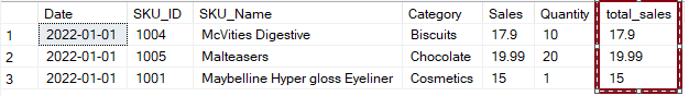
RANK( ) OVER(ORDER BY )
Suppose you want to rank( ) the transactions by their sales amount for each of the rows, we can use RANK( ) function along with OVER( ) clause.
OVER( ) clause is always used with RANK( ) functions as it means you are iterating over all the rows in the data.
ORDER BY clause inside OVER( ) clause indicates that the rows should also be sorted / ordered.
SELECT * , rank() over(ORDER BY sales)
FROM sales_table;
In the following output, last column represents the rank for each row. Note that the entire data is sorted in ascending order for sales column. Row with lowest sales is ranked 1 and highest sales is ranked highest (i.e., 11) .
One thing to notice that for rows 1 and 2 (circled in red) since they have the same sales, thus, their rank is also same i.e., 1. But in row 3, the rank is now 3 and not 2. Thus in case of ties, the same rank is allocated to tied rows, but the next rows will have their rank skipped by number of ties.

Ranks in descending order
Task: Calculate the rank( ) for transactions by sales, but ordered in descending order.
To calculate the ranks in descending order (i.e., item having highest sale should have rank 1 and lowest sales should have rank 11) , in ORDER BY statement we define the keyword DESC.
SELECT * , rank() over(ORDER BY sales DESC)
FROM sales_table
DENSE_RANK( )
Earlier we noticed that in case of ties the ranks get skipped for future rows. However, if you do not want to skip the rank then you can use DENSE_RANK( )
SELECT * , dense_rank() over(ORDER BY sales DESC)
FROM sales_table;
In the output below you can see that rows 1 and 2 are tied as rank 1, but row 3 has now rank 2 because we have used dense_rank( ) . If we use rank( ) function then its rank would have been skipped to 3.

ROW_NUMBER( )
To get the row number for each row, we can use ROW_NUMBER( ) function along with OVER( ) and ORDER BY( ) clauses. Thus, row_number function can be considered as giving different ranks in case of ties.
In the code below we are using ORDER BY clause for sales in descending order and calculating the row_number.
SELECT * , row_number() over(ORDER BY sales DESC)
FROM sales_table;
In the output below it can be seen that last 2 rows have same amount of sales, but their ranks are different.

RANK functions OVER , PARTITION BY and ORDER BY together
In the tutorial above we have seen that PARTITION BY( ) clause is used to partition / divide the data on the basis of a categorical column and then the calculations are performed. Similarly, partition y clause can be used along with rank functions like rank( ) , dense_rank( ) , row_number( )
Task: Calculate different ranks, ignoring the ties for various categories, on the basis of sales in descending order.
SELECT * , row_number() over(partition by category ORDER BY sales DESC)
FROM sales_table;
In the following output we can see that the data has been partitioned by 4 categories and the ranks have been calculated independently for each category.
Since we want to ignore the ties, thus using row_number has helped us by giving different ties to each observation for each category (see row 2 and 3 - they have both the same sales belonging to same category).
Also note, that the sales for each category are sorted / ordered in descending order.

ROWS BETWEEN
To calculate the cumulative sales or lags and leads we have the following keywords to be used in the window functions.
PRECEDING
FOLLOWING
UNBOUNDED PRECEDING - All the rows preceding the current row
UNBOUNDING FOLLOWING - All the rows after the current row
CURRENT ROW
Cumulative Sum
To calculate the cumulative sum, we need the sum of sales for all the rows before our current row and current row, thus we specify the ROWS BETWEEN
UNBOUNDED PRECEDING and CURRENT ROW with OVER clause.
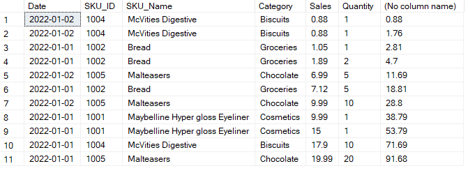
SELECT *, sum(sales) OVER(ORDER BY sales ROWS BETWEEN unbounded preceding and current row)
FROM sales_table;
In the output below, you can see that in the last column, for each row SQL created a window (i.e., a subset of the dataset) for that row and all its preceding rows. Then SQL calculates the sum. Since we have 11 rows in our data, thus 11 windows were created to calculate 11 different cumulative sums.
Task: Calculate the Cumulative Sales for each day
To calculate the cumulate sales for each day we need to partition our data with the date column, and then calculate the cumulative sum using OVER( ) function and Rows between unbounded preceding and current row.
SELECT *, sum(sales) over(partition by date order by date rows between unbounded preceding and current row)
FROM sales_table;
LAGS
To get 1 value before our current row (i.e., lag values) we can use ROWS BETWEEN 1 preceding and 1 preceding and calculate the sum(sales) i.e., we take only 1 row preceding the current row and retrieve its sales amount.
Note that in the code below we have partitioned the data by date column thus, lag value for first transaction will not be available.
SELECT *, sum(sales) over(partition by date order by date rows between 1 preceding and 1 preceding)
FROM sales_table;
LEAD
To get the next value after our current row (i.e., lead values) we can use ROWS BETWEEN 1 FOLLOWING and 1 FOLLOWING and calculate the sum(sales) i.e., we take only 1 row following the current row and retrieve its sales amount.
Note that in the code below we have partitioned the data by date column thus, lead value for last transaction on the day will not be available.
SELECT *, sum(sales) over(partition by date order by date rows between 1 following and 1 following)
FROM sales_table;
NTILE
Ntile( ) window function divides the data into number of tiles (i.e., equal parts) specified by the user. i.e., NTILE( 3) will divide the data in 3 almost equal parts.
Note that NTILE( ) function requires an ORDER BY( ) clause with OVER( ) statement.
The following code creates 3 different divisions of our data: 1st part and 2nd part contain 4 rows each and last part contains 3 rows.
SELECT * , NTILE(3) OVER(ORDER BY sales )
FROM sales_table;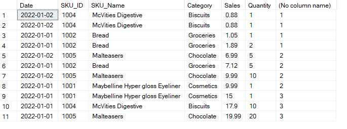
It is also possible to use NTILE with PARTITION BY clause as well.
Comments