Hierarchical Clustering
- Ekta Aggarwal
- Aug 18, 2022
- 5 min read
Hierarchical clustering is one of the popular unsupervised learning clustering methods. In this tutorial we would be covering the explanation of the algorithm in detail.
To understand, let us say we have N (say 100) observations. Initially each observation is a cluster of its own. Then we take pairwise distances (say, Euclidean distances) for each of the points. The pair which is closest to each other merges to form a cluster, thus we will have N-1 (i.e., 99) clusters and this process is repeated till we get our clusters.
To learn how to implement Hierarchical Clustering in Python you can refer to this article: Hierarchical Clustering in Python.
Algorithm for hierarchical clustering are either:
1. agglomerative in which we start at the individual leaves and successfully merge clusters together. It represents a 'bottom up' approach where each unit is its own cluster and a pair of clusters are merged as we move up the hierarchy.
2. divisive in which we start at the root i.e., consider all observations as a single cluster and recursively split the cluster. It is a 'top down' approach where all units start in one cluster and splits are performed as we move down the hierarchy.
Most widely agglomerative hierarchical clustering is used, thus for this lesson our scope is limited to agglomerative hierarchical clustering only.
Now let us understand a few concepts:
Distance matrix:
Say we have N points (p1, p2, ..., pN) in our data, thus we calculate the Euclidean distance for all the possible N X N pairs, say d12 for points p1 and p2; d13 for points p1 and p3.
Such a matrix is known as distance matrix, which will be used to determine which points are similar to each other, so that we can merge them to form a cluster.
Dendogram:
A dendogram is a diagram which is created with the distance matrix, and tells us how the clusters are formed.
The below image represents a dendogram of 8 points.

Each points (p1, p2, ... , p8) at the bottom of the dendogram are called leaves.
Leaves are combined to form small branches, as shown in the image below. Small branches are combined into larger branches until one reaches the top of the tree, representing a single cluster containing all the points.
The image below illustrates that points p1 and p2 we initally joined to form a cluster (say C1), then points p4 and p5 formed a cluster (say C2).
Then Cluster C1 (points p1 and p2) is combined with point p3 to form a bigger cluster.
Similarly all the clusters are formed.

Why is dendogram important?
Bu cutting the dendogram by a horizontal line, at different levels, we will get different number of clusters.
We can see in the below image that
if we cut our dendogram with a green line, then we will get 2 clusters, Cluster 1 with points p1,p2,.., p6 and Cluster 2 with points p7 and p8
if we cut our dendogram with an orange line, then we will get 3 clusters, Cluster 1 with points p1,p2,p3, Cluster 2 with p4, p5, p6 and Cluster 3 with points p7 and p8
Similarly blue line would divide our data in 4 clusters., Where cluster 3 and 4 will have only one single point i.e., p7 and p8 respectively.

How to decide the number of clusters with a dendogram?
Dendogram is important as it also helps in deciding the number of clusters.
In a dendogram, Y-axis represents the Euclidean distance.
To get the ideal number of clusters, we would
1. Extend the horizontal bars of the branches in the dendogram, depicted as blue dotted line in the image below.
2. Now we will see which is the largest distance which is not cut by these hypothetically extended blue dotted lines.
3. In the image below we see that topmost green bar is our largest Euclidean distance which has not been cut by any of these blue lines.

4. Now we will cut this largest Euclidean distance by any hypothetical line (red dotted line) to give us our clusters. Here we can see that for the below data we have got 2 clusters.

Hierarchical Clustering Algorithm:
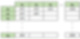
Step 1: Initially each data point forms a cluster. Let us say we have 5 points. which will make 5 clusters, C1, C2, C3, C4, and C5
Step 2: Compute the distance matrix / proximity matrix b/w all the clusters.

Step 3: Merge the 2 closest clusters.
Suppose C1 and C5 are the closest clusters. Thus they will be combined in a single cluster
Thus, number of clusters will reduce by 1

Step 4: Update the distance matrix for all the clusters. In the updated matrix, we will have 1 less row.

Step 5: Repeat steps 3 and 4 until only a single cluster remains.
How to measure this distance and similarity?
To measure the similarity we will use Euclidean distances between two points. We form the pairs of points such that 1 point belonging to cluster Ci and other point belonging to cluster Cj. However, there are various ways in which clusters can be formed:
Single link / Closest Link.
For single link / closest link we take the similarity between 2 clusters i.e., between clusters Ci and Cj and these clusters are merged if they have maximum similarity, which means the Euclidean distance should be the least.
Let us suppose point x belongs to cluster Ci, and y belongs to cluster Cj. sim denotes the similarity
i.e., sim(Ci, Cj) = max sim(x,y)
This method can lead to long and thin clusters, which might not be appropriate.

2. Complete Link / Furthest Link
For Complete Link / Furthest Link we take the similarity between 2 clusters i.e., between clusters Ci and Cj and these clusters are merged if they have minimum similarity, which means the Euclidean distance should be the maximum.
Let us suppose point x belongs to cluster Ci, and y belongs to cluster Cj. sim denotes the similarity
i.e., sim(Ci, Cj) = min sim(x,y)
This method can lead to spherical clusters which are generally appropriate.

Drawback: However, this method is highly sensitive to outliers as they are far away. Thus if one object is a cluster which is far away from other objects then it will highly influence the similarity.
3. Average Link
Average Link considers the average of similarity between the pairs of elements in the clusters.
sim(Ci,Cj) = ∑ sim(x,y)/|Ci|*|Cj|
This method is less susceptible to outliers.
4. Centroid Link
Firstly it will compute the centroids of the 2 clusters, and then willl merge the clusters on the basis of the centroids. However, this method is less popular.
5. Ward's Method
Just like Average Link, Ward method also considers the average similarity, however it takes the squared similarity. This method is widely popular.
sim(Ci,Cj) = ∑ sim(x,y)/|Ci|*|Cj|
To get the best clusters it is suggested to experiment with different linkage criteria and with a business sense you can get the best clusters.
Important points to be kept in mind!
1. Hierarchical Clustering evaluates the distance matrix, which is a time consuming process, thus for large datasets, this method is not recommended due to high run time. As a result, for large datasets K-means clustering is preferred as compared to Hierarchical Clustering.
2. Clustering methods are known to be sensitive to outlier. Thus, presence of outliers can impact the formation of clusters.
3. Standardisation of variables: If variables have very different scales (say age and salary, where age is generally < 100 while salary is in thousands) then we need to standardise the variables so that they have a similar mean and variance.
To learn how to implement Hierarchical Clustering in Python you can refer to this article: Hierarchical Clustering in Python.