Pandas Demystified!
- Ekta Aggarwal

- Jan 29, 2021
- 17 min read
Updated: Feb 14, 2022
Pandas is one of the most powerful Python libraries which make it a programmer's choice! It is built over Numpy and matplotlib and is used for data manipulations.
In this tutorial we will learn with plethora of examples to understand how data can be wrangled!
Key topics covered:
Reading a dataset:
In this tutorial we will make use of following CSV file:
Let us read our file using pandas' read_csv function. Do specify the file path where your file is located:
import pandas as pd
mydata = pd.read_csv("C:\\Users\\Employee_info.csv")
Viewing only first or last N rows.
head( ) function
In Python head( ) function is used to view first N rows. By default head( ) returns first 5 rows.
mydata.head()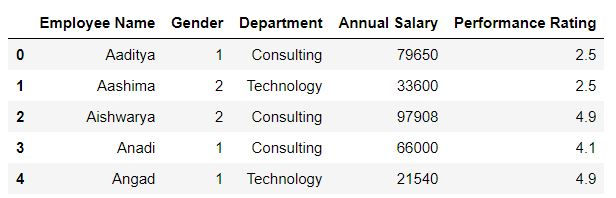
We can modify the number of rows in head( ) . In the following code, I have specified that I want to view first 2 rows only.
mydata.head(2)
tail( ) function
tail( ) function is used to view last N rows. By default tail( ) returns last 5 rows.
mydata.tail()
In the following code, we have specified that we want to view last 2 rows only.
mydata.tail(2)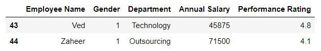
What is the shape of my data?
Shape of a data defines the number of rows and columns.
Using shape function we can get the shape of our mydata/
mydata.shapeOutput : (45, 5)
Shape function returns 2 values: where first value (value at index 0 ) is the number of rows, while second value (value at index 1) denotes the number of columns.
Following code returns the number of rows.
mydata.shape[0]Output: 45
By specifying [1] with shape, we can get the number of columns.
mydata.shape[1]Output: 5
Knowing our data's structure
We can get the column names using columns function as follows:
mydata.columnsOutput:
Index(['Employee Name', 'Gender', 'Department', 'Annual Salary ', 'Performance Rating'], dtype='object')
Row names are referred as index in Python. Using index function one can get the row names of the data.
mydata.indexOutput:
RangeIndex(start=0, stop=45, step=1)
*Range (0,45) means a counting from 0 to 44 (45 is excluded)
dtypes function
We can understand the type of our data using dtypes function
mydata.dtypesIn the following output 'object' means character;
int64 means integer
and float64 means float (decimal)values
are there in the corresponding column.
Output:
Employee Name object Gender int64 Department object Annual Salary int64 Performance Rating float64 dtype: object
astype function
We can change the type of our columns using astype function.
In the following code we are converting annual salary to a float.
mydata['Annual Salary '] = mydata['Annual Salary '].astype(float)mydata['Annual Salary '].dtypesOutput: dtype('float64')
Unique
unique function
To get the unique values in a column we can use unique function
Task: Get the unique department names in mydata.
mydata.Department.unique()Output: array(['Consulting', 'Technology', 'Outsourcing'], dtype=object)
nunique function
To count the number of unique values we have nunique function
Task: Count the unique department names in mydata.
mydata.Department.nunique()Output: 3
Getting a frequency distribution:
value_counts
Using value_counts one can get the frequency distribution of a variable.
For eg. In mydata for department columns: Consulting is appearing 17 times, Technology 17 times and outsourcing 11 times.
mydata.Department.value_counts()Output:
Consulting 17 Technology 17 Outsourcing 11 Name: Department, dtype: int64
We can sort the data on the basis of frequency in ascending order by specifying ascending = True.
mydata.Department.value_counts(ascending=True)Output:
Outsourcing 11 Technology 17 Consulting 17 Name: Department, dtype: int64
crosstab
Using crosstab one can get the frequency distribution of 2 variables.
pd.crosstab(mydata.Department,mydata.Gender)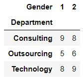
Selecting only numeric or character columns
_get_numeric_data
To get only numeric columns in our data we can use _get_numeric_data( ) function
numeric_only = mydata._get_numeric_data()
numeric_only.head()
Alternatively
select_dtypes :
By specifying exclude = 'object' (i.e. excluding character columns) we can get the numeric columns.
numeric_only = mydata.select_dtypes(exclude='object')
numeric_only.head()
By specifying include = 'object' we can get the character columns.
character_only = mydata.select_dtypes(include='object')
character_only.head()
To get numeric columns we can select multiple dtypes by providing the list as follows:
import numpy as np
numeric_only = mydata.select_dtypes(include=['int','float',np.number])
numeric_only.head()
Dropping rows or columns using drop( )
Using drop function we can drop rows and columns from our data.
Task: Drop department columns from our data.
mydata.drop('Department',axis = 1).head()Alternatively, you can specify axis = 'columns' to delete the column.
mydata.drop('Department',axis = "columns").head()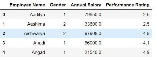
Dropping multiple columns:
To drop multiple columns we specify the list of columns to be deleted:
Task: Drop the columns department and gender from mydata
mydata.drop(['Department','Gender'],axis = "columns").head()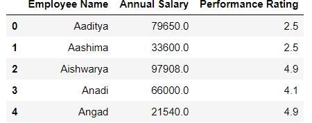
Dropping rows:
To drop rows from our data we specify axis = 0 or axis = "index"
Task: Drop first 10 rows from mydata
mydata.drop(range(10),axis = "index").head()Alternatively,
mydata.drop(range(10),axis = 0).head()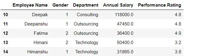
Renaming columns in a dataframe
Let us create a copy of our dataset as mydata_copy.
mydata_copy= mydata.copy()Renaming all the columns
We can fetch the column names as follows:
mydata_copy.columnsOutput:
Index(['Emp Name', 'Sex', 'Dept', 'Salary', 'Rating'], dtype='object')
To rename all the columns we can assign a list of new column names as follows:
Note: The column names must be in exact order as the previous column names
mydata_copy.columns = ['Name','Gender','Dept','Salary','Rating']mydata_copy.head(2)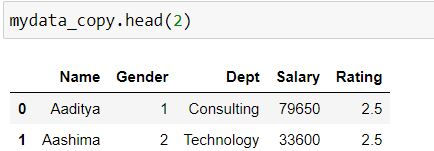
Renaming only some of the columns
To rename only some of the columns we use rename( ) function. In rename( ) we define columns = {our dictionary of key-values}
Keys are Old column names
Values are New column names
Let us rename columns Name and Gender to Emp Name and Sex respectively.
mydata_copy.rename(columns={"Name" : "Emp Name","Gender" : "Sex"})
By default inplace = False which means the changes won't be made in original dataset. Thus we need to save the new data.
To make changes in original data we set inplace = True.
mydata_copy.rename(columns={"Name" : "Emp Name","Gender" : "Sex"},inplace = True)mydata_copy.columnsOutput
Index(['Emp Name', 'Sex', 'Dept', 'Salary', 'Rating'], dtype='object')Creating new columns in a dataframe
Let us create a copy of our dataset as mydata_copy and rename our columns.
mydata_copy= mydata.copy()
mydata_copy.columns  = ['Name','Gender','Dept','Salary','Rating']
Let us create new column Monthly_Salary = Salary/12
Using square brackets [ ]:
To create a new colujmn we need to define new column name in [ ] square brackets. and define our formula as follows:
mydata_copy['Monthly_Salary'] = mydata_copy['Salary']/12Note: We cannot create new columns by defining data_name.new_column_name. We MUST use [ ] square brackets to create new columns.
Following code will lead to an error.
mydata_copy.Monthly_Salary_exp= mydata_copy['Salary']/12
Using eval function:
In the eval function we can specify our column names directly without mentioning the name of our data repeatedly.
In the LHS, we have used eval( ) function i.e. we will not need to write mydata_copy['column name'] .
mydata_copy['Monthly_Salary2'] = mydata_copy.eval('Salary/12')Using assign function:
If we have to create multiple columns then we can use assign function as follows:
Syntax:
new_data= old_data.assign( new_col_1= calculation_for_new_col1, new_col_2 = calculation_for_new_col2)
mydata_copy2 = mydata_copy.assign(Monthly_Salary3 = mydata_copy.Salary/12)mydata_copy2.head(3)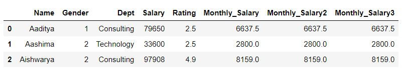
Filtering data
Filtering with loc
To filter the data with loc we need to provide the column or index names!!!!!
Basic sytax for filtering:
For filtering the data we need to provide 2 positions separated by a comma inside a comma i.e .[ a,b] where a denotes the row names or Boolean vector for rows, while b is the column names or Boolean vector for columns. To select all the rows or all the columns we denote it by a colon ( : )
Task: Filter the data for all the rows and 2 columns: Employee name and gender.
Since we are selecting all the rows thus we have written a colon ( :) instead of 'a'.
To select multiple columns we have providing our list ['Employee Name','Gender'] in place of 'b'
mydata.loc[:,['Employee Name','Gender']]Task: Filter the data for first 5 rows and 2 columns: Employee name and gender.
Since we are selecting first 5 rows only thus we have defined our range 0:5 in place of 'a' which means start from row 0 till row 4 (5 is excluded)
mydata.loc[0:5,['Employee Name','Gender']]Alternatively
range(5) means 0:5 (i.e. 5 is excluded)
mydata.loc[range(5),['Employee Name','Gender']]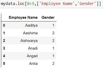
Task: Filter the data for first 5 rows and all the columns
mydata.loc[range(5),:]Filtering for consecutive columns:
To select consecutive columns we can write columnName1 : columnNameN by which all columns starting from columnName1 till columnNameN will be selected.
Task: Filter first 5 rows and columns from employee name till annual salary.
Here we have written "Employee Name" : "Annual Salary " to retrieve all the column between them (including both of them)
mydata.loc[range(5),"Employee Name" : "Annual Salary "]Filtering using Boolean vectors.
Task: Filter the data for the rows where gender is 1.
In the below code mydata.Gender == 1 returns a Boolean vector which takes the value True when gender is 1, otherwise False.
Wherever our Boolean vector has True, only those rows will be selected.
mydata.loc[mydata.Gender == 1,:]Filtering for multiple conditions
AND condition - when multiple condition need to be true
Task: Filter the data for the rows where gender is 1 and department is consulting.
In the below code (mydata.Gender == 1) & (mydata.Department == 'Consulting') returns a Boolean vector which takes the value True when both gender is 1 and Department is consulting, otherwise False.
mydata.loc[(mydata.Gender == 1) & (mydata.Department == 'Consulting'),:]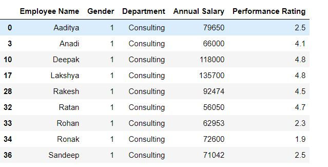
Task: In the above query select only employee name and salary
mydata.loc[(mydata.Gender == 1) & (mydata.Department == 'Consulting'),['Employee Name','Annual Salary ']]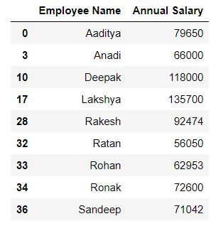
OR condition - when at least one condition needs to be true
Task: Filter the data for the rows where either gender is 1 or Salary is more than 110000.
Since we need to apply an 'or' condition i.e. at least one of the conditions should be true thus in Python we use '|' to denote 'or'
mydata.loc[(mydata.Gender == 1) | (mydata['Annual Salary '] > 110000),['Employee Name','Annual Salary ']]IN CONDITION
Task: Filter for rows where department is either consulting or outsourcing.
We can achieve this using or '|' condition as follows:
mydata.loc[(mydata.Department == 'Outsourcing') | (mydata.Department == 'Consulting'),:]But suppose we have to choose for multiple values (say 10 departments) then writing OR condition would be too tedious.
To simplify it we have .isin( ) function in Python. Inside isin( ) we specify the list of values which need to be searched.
In the following code we have written mydata.Department.isin(['Outsourcing','Consulting']) i.e. this will return a Boolean vector where department name is either outsourcing or consulting.
mydata.loc[mydata.Department.isin(['Outsourcing','Consulting']),:]Excluding the rows satisfying a particular condition
Task: Filter for rows where department is neither consulting nor outsourcing.
It means we do not want the department names to be consulting and outsourcing. To do this, we can firstly create a vector using .isin( ) which will return True where department is consulting or outsourcing, and then specify to exclude such rows i.e. provide negation.
To provide a negation we write a (~) symbol before the Boolean vector.
mydata.loc[~mydata.Department.isin(['Outsourcing','Consulting']),:]pd.query
We can filter our rows using pd.query( ) function
Task: Filter for rows where Gender is 1.
mydata.query('Gender ==1')Filtering with iloc
To filter the data with iloc we need to provide the column or index names!!!!!
Task: Filter for first 5 rows. (Since our index names are 0:44, thus iloc and loc lead to same output)
mydata.iloc[range(5)]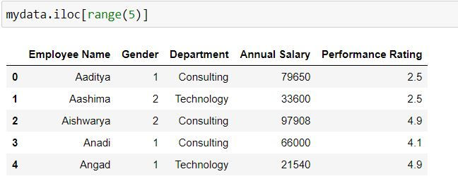
Task: Filter for first 5 rows and first 3 columns.
To filter for first 3 columns we have defined 0:3 after comma.
mydata.iloc[0:5,0:3]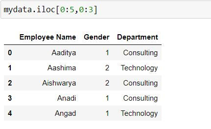
Obtaining indices using np.where
Task: Filter for rows where department is consulting.
Numpy's where function returns the indices wherever a particular condition is found True. We can then use those indices in iloc to filter the rows.
import numpy as npnp.where(mydata['Department'] == 'Consulting')Output:
(array([ 0, 2, 3, 7, 8, 10, 17, 19, 21, 25, 28, 31, 32, 33, 34, 36, 41], dtype=int64),)
mydata.iloc[np.where(mydata['Department'] == 'Consulting')]
Managing index in a dataframe.
Setting the index in an already existing dataset
Using set_index( ) we can set our index in already existing dataset.
data1 = mydata.set_index(["Employee Name","Gender"]).sort_index()data1.head(10)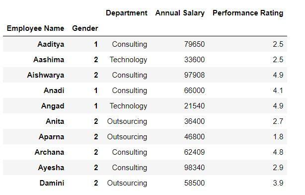
Resetting the index
We can also reset the index i.e. make them columns in our data using reset_index( ) function.
By default inplace = False, which means to save the changes we need to create a new dataset.
To make the changes in the original dataset we mention inplace = True
data1.reset_index(inplace = True)
data1.head()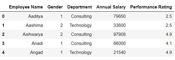
To learn more about how to deal with index for filtering them refer to this tutorial:
Sorting the data
We can sort the data on the basis of a single column using sort_values( ) function
Task: Sort mydata by Annual Salary
mydata.sort_values("Annual Salary ",ascending = False)By default ascending = True and inplace = False. To sort the data in descending order we need to specify ascending = False. To make the changes in original data you need to set inplace = True, otherwise you need to save your data in a new dataset.
Sorting data by multiple variables
Task: Sort mydata by Department and Annual Salary
mydata.sort_values(['Department',"Annual Salary "],ascending = False)Task: Sort a single column: Annual Salary
mydata['Annual Salary '].sort_values()Ranking the data
Let us firstly create a copy of our dataset:
data3 = mydata.copy()To provide ranks to a dataset we can use rank( ) function.
By default ascending = True which means lowest value will be provided rank 1.
data3['Rank_of_salary']  = data3['Annual Salary '].rank(ascending=True)

data3.head()
Ranking and group by
Task: Provide ranks on the basis of annual salary within each department.
In the following code we have grouped our annual salary by department and then have applied rank( ) function. Note: we have kept ascending = False.
data3['Rank_by_department'] = data3['Annual Salary '].groupby(data3.Department).rank(ascending =False)Let us filter the above data for consulting department:
consulting = data3.loc[data3.Department == 'Consulting',:]Using sort_values( ) function let us sort the data by rank and observe the output.
consulting.sort_values('Rank_by_department')Getting descriptive statistics
describe( ) function
We can get basic summary statistics for our data using describe( ) function
mydata.describe()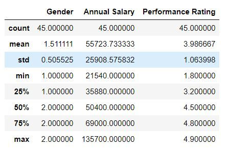
By default describe returns summary statistics for numeric columns. To get summary statistics for character or categorical column we need to specify include ='object'
mydata.describe(include='object')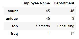
To get only one statistic(say mean) we can calculate it as follows:
mydata.mean()Output:
Gender 1.511111 Annual Salary 55723.733333 Performance Rating 3.986667 dtype: float64
Task: Calculate median for all numeric columns in mydata
mydata.median()Output:
Gender 2.0 Annual Salary 50400.0 Performance Rating 4.5 dtype: float64
Task: Calculate average annual salary using mydata.
mydata['Annual Salary '].mean()Output: 55723.73333333333
Task: Calculate average annual salary and performance rating using mydata.
mydata[['Annual Salary ','Performance Rating']].mean()
mydata.loc[:,['Annual Salary ','Performance Rating']].mean()
Output:
Annual Salary 55723.733333 Performance Rating 3.986667 dtype: float64
agg function
We can calculate multiple summary statistics using agg( ) function.
Task: Calculate mean and median for all the columns.
mydata.agg(['mean','median'])
Task: Calculate mean and median for annual salary and performance rating,
mydata[['Annual Salary ','Performance Rating']].agg(['mean','median'])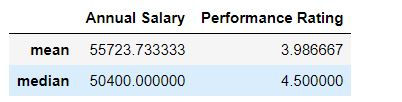
Task: Calculate mean and median for annual salary and minimum and maximum performance rating.
For this we can define a dictionary where keys are the column names and values are the list of statistics for the corresponding keys.
Eg. We have the key as Annual Salary and its values are ['mean' , 'median'] ( a list)
mydata.agg({"Annual Salary " : ['mean','median'], "Performance Rating" : ['min','max']})
Group by
Task: Retrieve the minimum value for all the variables for each department.
Since we want to divide our data on the basis of each department and then get the minimum values, for this we have grouped our data by department and then applied the min( ) function to get minimum values for all the columns.
mydata.groupby('Department').min()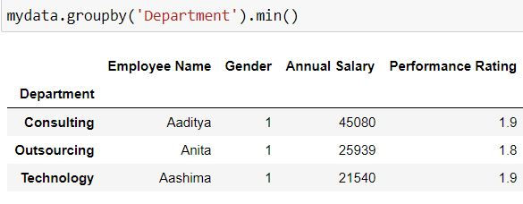
Grouping by multiple variables
Task: Retrieve the minimum value for all the variables for each department and gender.
Here have specified 2 variables Department and Gender in our group by
mydata.groupby(['Department','Gender']).min()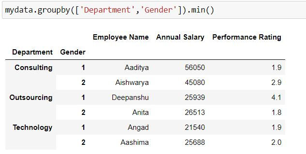
By default group by is returning minimum values for all the columns. To fetch minimum values for a single column (say Annual Salary ), after group_by we select the column name and then calculate the summary statistic.
mydata.groupby(['Department','Gender'])['Annual Salary '].min()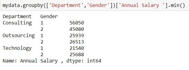
Calculating multiple summary statistics:
Task: Calculate mean and median values for each Department and Gender combination.
To calculate multiple summary statistics we can use agg( ) function. Inside agg we have defined the summary statistics which we want to retrieve.
mydata.groupby(['Gender','Department']).agg(['mean','median'])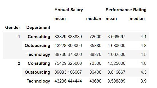
To learn more about group by in detail you can refer:
Calculating Percentiles
Using quantile( ) function we can get percentiles or quantiles for our data.
Task: Calculate 1st quartile or 25th quantile for all the variables.
mydata.quantile(0.25)Output:
Gender 1.0 Annual Salary 35880.0 Performance Rating 3.2 Name: 0.25, dtype: float64
Task: Calculate 25th,40th, 8th and 99 quantile for all the variables.
mydata.quantile([0.25,0.4,0.8,0.99])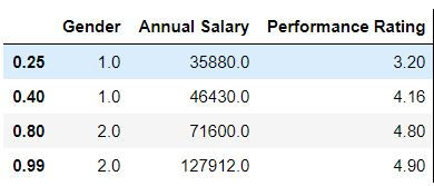
Task: Calculate 25th,40th, 8th and 99 quantile for annual salary
mydata['Annual Salary '].quantile([0.25,0.4,0.8,0.99])Output:
0.25 35880.0 0.40 46430.0 0.80 71600.0 0.99 127912.0 Name: Annual Salary , dtype: float64
Cumulative sum
Let us firstly sort our data by department and annual salary. (We have sorted salaries in ascending order)
dummydata = mydata[['Department','Annual Salary ']].sort_values(['Department','Annual Salary '], ascending = [True,False])We can calculate cumulative sum using cumsum( ) function.
Task: Calculate cumulative sum for the above data.
dummydata['Annual Salary '].cumsum()Group by and cumulative sum
Task: Calculate cumulative sum for each department.
For this we have firstly used groupby( ) command and then applied cumsum( ) function.
dummydata['Department_wise_cumsum'] = dummydata.groupby('Department').cumsum()
dummydata
Dealing with missing values
A missing value can be created using Numpy's .nan function. So let us firstly import Numpy as np
import numpy as npDataset:
Let us create a dataset where missing values are created by np.nan
data1 = {'Product_category': ['Makeup', 'Biscuits', 'Household_Cleaning', 'Cold_drinks'],
        'Sales': [10000, 2000, 17891, np.nan],
        'Returns' : [678, np.nan, 678,234]}

data1 = pd.DataFrame(data1)
data1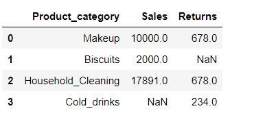
isnull ( ) function
isnull( ) function returns True when a missing value is encountered, otherwise returns False.
data1.isnull()For index 1 and 3 we have Returns and Sales value as True respectively.

Applying isnull( ) on a column
data1.Sales.isnull()In the data, in sales column we had a missing value at index =3 thus we have a True at that position.

Filtering for rows having missing values.
Task: Filter for rows where Sales values are missing.
We can filter the rows using .loc and apply our Boolean vector of True and False (which we have got the in the previous code)
data1.loc[data1.Sales.isnull(),]
notnull ( )
notnull is complementary of isnull( ) .When the data is missing then notnull( ) returns a False, while for non-missing data it returns True.
Filtering for rows having non-missing values.
Task: Filter for rows where Sales values are not missing.
We can filter the rows using .loc and apply our Boolean vector of True and False i.e. data1.Sales.notnull()
data1.loc[data1.Sales.notnull(),]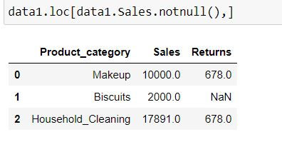
Getting total number of missing values.
Using sum( ) and isnull( ) function we can get the total number of missing values in a column
sum(data1.Sales.isnull())
data1.Sales.isnull().sum() #Alternatively
Output: 1
Getting total number of non-missing values.
Using sum( ) and notnull( ) function we can get the total number of non-missing values in a column
sum(data1.Sales.notnull())
data1.Sales.notnull().sum()
Output: 3
Filling missing values
We can fill missing value in a data using fillna( ) function.
data1.fillna(value="Missing")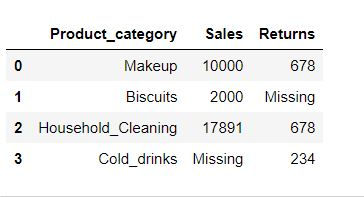
Dropping missing values
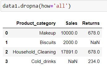
Using dropna( ) function we can drop the rows having missing values.
By specifying how = 'all' we are telling Python to delete the rows where all of the columns have missing values (that is entire row is full of NaN)
data1.dropna(how='all')Since we did not have any row where all columns have missing values thus no row got deleted.
By specifying how = 'any' we are telling Python to delete the rows where at least one missing is present.
data1.dropna(how='any')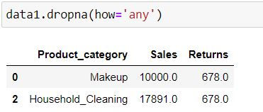
In the above 2 codes we are considering all the columns for missing values. To consider only some of the columns we define subset = ['list of columns to be considered']
For the code chunk below, those rows will be deleted where there is missing value is Sales column.
data1.dropna(subset = ['Sales'],how = 'all')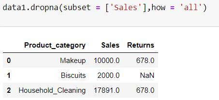
In the following code, those rows will get deleted where there is missing value in either of the 2 columns (as how = "any")
data1.dropna(subset = ['Sales','Returns'],how = 'any')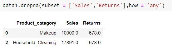
inplace = True
By default Python does not make changes in the original dataset as inplace = False. To make changes in the original data we need to specify inplace = True
data1.dropna(subset = ['Sales','Returns'],how = 'all',inplace = True)
data1
Dealing with duplicate values
Let us create a dataset which we will use
data = pd.DataFrame({
"Product_Category" : ["Makeup","Makeup","Makeup","Cold_drinks","Sauces","Sauces"],
"Sales" : [15000,15000,10000,23454,7800,9000]})
data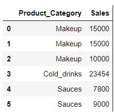
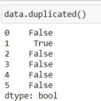
duplicated( ) function
Pandas' duplicated( ) function when used with a dataframe returns a boolean series where True indicates that entire row has been duplicated.
data.duplicated()In the above dataset our row at index 1 (second row) is a duplicate thus duplicated( ) has returned a series where second element is True and rest are False (False denotes that the value is a unique value)
We can use the above boolean series to filter our dataset: To get a dataset with only duplicates :
data.loc[data.duplicated(),:]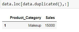
By default Python considers first occurence as unique occurence (ie. row with index 0) and all other repetitions as duplicates (row with index 1). This is because by default keep = "first" in duplicated( ) function.
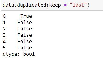
To keep the last occurrence as unique and all others as duplicate we set keep = "last"
data.duplicated(keep = "last")Note that now row with index 0 has True (i.e. it is a duplicate) while row with index 1 is False (it is being considered as unique)
data.loc[data.duplicated(keep = "last"),:]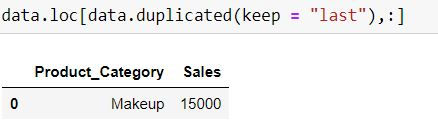
When keep = False then Python treat all of the repetitions (including first and last occurrence as duplicates)
data.duplicated(keep = False)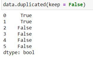
Dropping duplicate values
Using pandas' drop_duplicates( ) we can drop the duplicate values.
In the following code keep = "first" means first occurrence (at index 0 ) would be a unique value and hence would not be dropped.
data.drop_duplicates(keep = "first")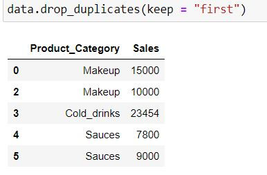
keep = "last" means last occurrence (at index 1) would be a unique value and would not be dropped.
data.drop_duplicates(keep = "last")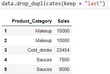
keep = False means all occurrence (at index 0 and 1) would be a treated as duplicates and hence would be dropped.
data.drop_duplicates(keep = False)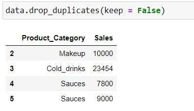
Finding duplicates on the basis of some columns:
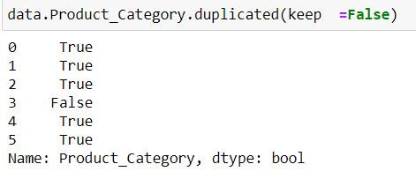
To find duplicated on the basis of Product_Category column we apply duplicated function to the single column and not on entire data:
data.Product_Category.duplicated(keep =False)Note: We have defined keep = False. Since Makeup and Sauces are repeated thus we have a True corresponding to their indices.
Task: Filter for those product categories which are unique.
In the code below we are filtering for duplicate product categories using duplicated( ) function and have then provided a negation using ' ~ ' symbol.
data.loc[~data.Product_Category.duplicated(keep =False),:]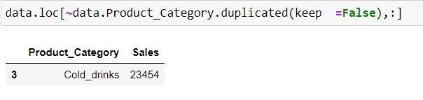
Creating pivot tables
We can create pivot tables using pandas' pivot_table function.
Syntax
data.pivot_table(values = "list of column names for aggregation ",
index = "List of categorical column for rows",
columns="List of categorical column for column",
aggfunc = [List of functions to be evaluated],
margins = [True or False for getting grand total i.e. margin],
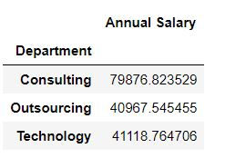
margins_name="Column name for Grand Total or Margins")Task 1: Get average salary for each department.
mydata.pivot_table(values = "Annual Salary ",index = "Department")By default Python calculates averages for numeric columns. Thus to get an average salary we have defined values = "Annual Salary "
We want to show the data for each department in rows : thus we defined index = "Department"
Task 2: Get median salary for each department.
To get median salary we have define aggfunc = np.median in the code below.
import numpy as np
mydata.pivot_table(values = "Annual Salary ",index = "Department",aggfunc = np.median)
Task 3: Get average and median salary for each department.
To calculate multiple statistics we have defined the list of functions [np.median , np.mean] in aggfunc
mydata.pivot_table(values = "Annual Salary ",index = "Department",aggfunc = [np.median,np.mean])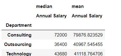
Task 4: Get average and median salary for each department and gender.
To create a 2X2 view of department and age we have defined columns = "Gender".
Note: If we wanted we could have specified index = ["Department" ,"Gender"] but that would have resulted in a long table instead of a 2X2 table.
mydata.pivot_table(values = "Annual Salary ",index = "Department",columns="Gender",aggfunc = [np.median,np.mean])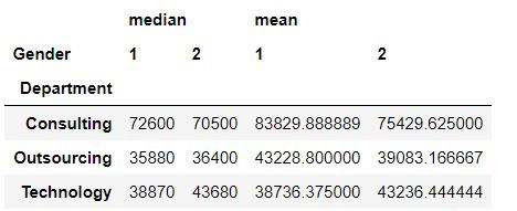
To learn about pivot tables in detail you can refer:
Creating dummy variables
To understand what are dummy variables in detail you can refer: What are dummy variables and creating dummy variables in Python.
Using pandas' get_dummies( ) function we can create dummy variables with a single line of code.
Let us create another copy of our data
data2 =mydata.copy()Using pandas' get_dummies( ) function we can create dummy variables with a single line of code.
For each department name have added a prefix "Dep"
pd.get_dummies(data2.Department,prefix = "Dep")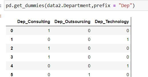
get_dummies( ) only creates dummy variables. To append it in our data we use pandas' concat function:
Let us firstly save our dummy variables in a dataset.
dummy_variables = pd.get_dummies(data2.Department,prefix = "Dep")We now concatenate our original data using pd.concat( ) , by defining axis = 1 or axis = "columns" we are telling Python to add the columns horizontally (and not append them as rows).
pd.concat([data2,dummy_variables],axis = 1)

#alternatively
pd.concat([data2,dummy_variables],axis = "columns")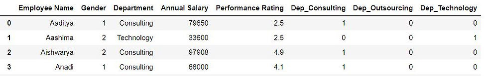
When Dep_Consulting = 1 and Dep_Technology is 0 then it is self-implied that dep_outsourcing will be 0. Thus in this case we only need 3-1 = 2 dummy variables. We can drop the first column by specifying drop_first = True.
dummy_variables = pd.get_dummies(data2.Department,prefix = "Dep",drop_first=True)

pd.concat([data2,dummy_variables],axis = "columns")
Merging or joining datasets
Let us consider 2 datasets data1 containing sales and data2 containing returns for various product categories
data1 = pd.DataFrame({
'Product_category': ['Makeup','Medicines','Syrups'],
'Sales': [20000,6200,70000]})
data2 = pd.DataFrame({
'Product_category': ['Makeup','Vegetables','Medicines'],
"Returns" : [2300,630,2400]})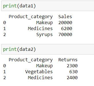
Inner Join
Inner Join takes common elements in both the tables and join them. By default pd.merge( ) returns inner join as output.
data1.merge(data2,on = "Product_category")alternatively, you can specify how = "inner"
data1.merge(data2,on = "Product_category",how ="inner")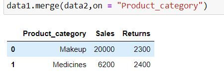
Output Explanation: Since both the data have only 2 product categories in common : Makeup and medicines thus we have only 2 rows in our output.
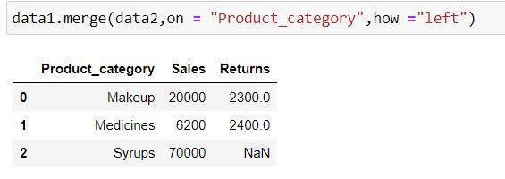
Left Join
Left join takes all the records from left table (specified before merge keyword) irrespective of availability of record in right table (specified inside parenthesis of merge)
If the record is not available in the right table then missing values get generated for such records.
data1.merge(data2,on = "Product_category",how ="left")Output Explanation: In data1 (left table) we have 3 product categories available thus we have only those 3 categories available in output. Since there is no information about Syrups in data2 (right table) thus we have NaN (missing values) generated for Returns for it.
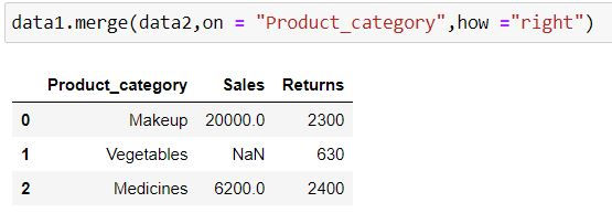
Right Join
Rihgt join takes all the records from right table (specified inside parenthesis of merge) irrespective of availability of record in left table (specified before merge keyword)
If the record is not available in the left table then missing values get generated for such records.
data1.merge(data2,on = "Product_category",how ="right")Output Explanation: In data2 (right table) we have 3 product categories available thus we have only those 3 categories available in output. Since there is no information about Vegetables in data1 (left table) thus we have NaN (missing values) generated for Sales for it.
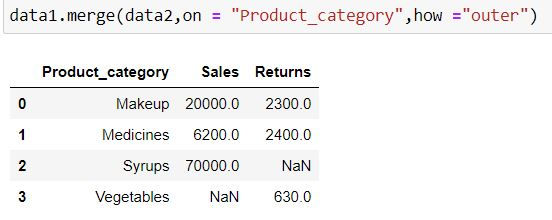
Outer Join or Full Join
Outer join or Full join takes all the records from both the tables. Missing values get generated if a record is available in only one table.
data1.merge(data2,on = "Product_category",how ="outer")Output Explanation: In data1 (left table) and data2 (right table) we have 5 unique product categories available thus we have 5 categories available in output.
Since there is no information about Syrups in data2 (right table) thus we have NaN (missing values) generated for Returns for it.
Similarly there is no Sales information available for Vegetables.
Anti - Join
Anti join comprises of those records which are present in one table but not in other.
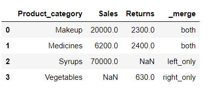
Let us firstly understand what is indicator =True means in merge( ) function:
data1.merge(data2, on = "Product_category",how = "outer",indicator=True)In _merge column following the meaning of its values:
both: Record is available in both the tables
left_only: Record is available only in left table(data1)
right_only: Record is available only in right table (data2)
Let us save this result in a new dataset called merged
merged = data1.merge(data2, on = "Product_category",how = "outer",indicator=True)Anti join 1:
In the following code we are fetching those rows which belong to DATA1 and are not present in DATA2 by filtering for rows where _merge column has values: "left_only"
merged.loc[merged["_merge"] == "left_only",:]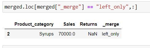
Output Explanation: In data1 (left table) Syrups is present whose information is absent in data2 (right table) thus we have only that row in the output.
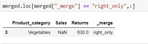
Anti join 2:
In the following code we are fetching those rows which belong to DATA2 and are not present in DATA1 by filtering for rows where _merge column has values: "right_only"
merged.loc[merged["_merge"] == "right_only",:]Output Explanation: In data2(right table) Vegetables is present whose information is absent in data1 (left table) thus we have only that row in the output.
To understand more about joins : one to many mapping, many to many mapping , when variables to be joined have different names etc. refer to this detailed tutorial:
Concatenating and appending datasets
Using pd.concat( )
Using pd.concat( ) we can append our data row-wise as well as column-wise.
Let us consider 3 datasets:
data1 = pd.DataFrame({'Product_category': ['Makeup','Medicines','Syrups'],
                         'Sales': [20000,6200,70000]})

data2 = pd.DataFrame({'Product_category': ['Biscuits','Vegetables','Fruits'],
                         'Sales': [18000,9000,30000]})

data3 = pd.DataFrame({'Product_category': ['Cold_Drinks','Chocolates','Books'],
                         'Sales': [14000,23000,14000]})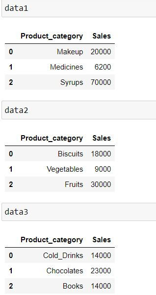
Let us concatenate the data. By default pd.concat( ) appends the data by rows.
pd.concat([data1,data2,data3])Note the indices for the resultant dataset: They are 0, 1 and 2. When another data is appended below it then indices are taken for another dataset.
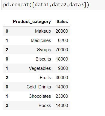
By default pd.concat( ) concatenates data by row. i.e. axis = "index" or axis = 0.
To add columns to the data we define axis = "columns" or axis = 1
pd.concat([data1,data2,data3],axis = "columns") #or axis = 1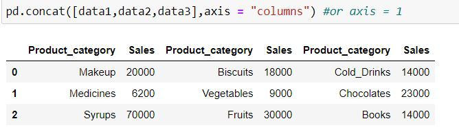
Using append( ) function
Pandas' append function is used only to append the datasets row-wise. You cannot append them column-wise.
Let us consider following 2 datasets:
data1 = pd.DataFrame({'Product_category': ['Makeup','Medicines','Syrups'],
                         'Sales': [20000,6200,70000]})

data2 = pd.DataFrame({'Product_category': ['Biscuits','Vegetables','Fruits'],
                         'Sales': [18000,9000,30000],
                     "Returns" : [2300,630,2400]})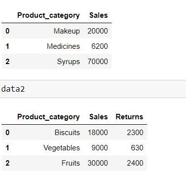
To learn in detail about various options available in pd.concat and pd.append( ) refer to this tutorial:


Comments